Compile Your Model

As a developer, you can use the ModelSDK to prepare machine learning models for deployment on the MLSoC. The process of preparing a model includes converting it to use lower-precision data types on which the MLSoC can compute much more efficiently. Developers have several options to do this conversion, depending on the computational performance and numerical accuracy they want their model to attain. Post-Training Quantization (PTQ) is an efficient and straightforward method to reduce model size and improve inference speed while maintaining minimal accuracy loss.

The PTQ workflow involves:

Loading a model
Quantizing it to int8 or int16
Evaluating its accuracy
Compiling it for execution

To achieve this, you will need to write a Python script to perform these steps.

The following example demonstrates step-by-step how to optimize a ResNet-50 model using PTQ.

Start by running this sample script in Palette to convert a ResNet-50 model into an optimized version using PTQ.

Download Sample Script

First, uncompress the example in the Palette environment and install necessary dependencies. Assuming the file was copied to the ~/workspace directory on the host, which maps to /home/docker/sima-cli by default.

Grant the RW permission to the pybind11-2.13.6.dist-info & pybind11 package to avoid any permission access issue

sima-user@docker-image-id:/home/$ cd docker/sima-cli

    sudo chmod 755 -R /usr/local/lib/python3.10/site-packages/pybind11-2.13.6.dist-info
    sudo chmod 755 -R /usr/local/lib/python3.10/site-packages/pybind11

Setup the downloaded project and install the required python packages in the virtual environment with access to system-site-packages

sima-user@docker-image-id:/home/$ cd docker/sima-cli
sima-user@docker-image-id:/home/docker/sima-cli$ tar -xvf ptq-example.tar.gz
    ptq-example/
    ptq-example/README.md
    ptq-example/src/
    ptq-example/src/x86_reference_app/
    ptq-example/src/x86_reference_app/resnet50_reference_classification_app.py
    ptq-example/src/modelsdk_quantize_model/
    ptq-example/src/modelsdk_quantize_model/resnet50_quant.py
    ptq-example/models/
    ptq-example/models/download_resnet50.py
    ptq-example/data/
    ptq-example/data/openimages_v7_images_and_labels.pkl
    ptq-example/data/golden_retriever_207.jpg
    ptq-example/data/imagenet_labels.txt
    ptq-example/requirements.txt

sima-user@docker-image-id:/home/$ cd /home/docker/sima-cli/ptq-example
sima-user@docker-image-id:/home/docker/sima-cli/ptq-example$ python3 -m venv --system-site-packages .env
sima-user@docker-image-id:/home/docker/sima-cli/ptq-example$ source .env/bin/activate
(.env)sima-user@docker-image-id:/home/docker/sima-cli/ptq-example$ pip3 install -r requirements.txt

Then, run the download_resnet50.py script to retrieve the official resnet50 ONNX model.

(.env)sima-user@docker-image-id:/home/$ cd /home/docker/sima-cli/ptq-example/models
(.env)sima-user@docker-image-id:/home/docker/sima-cli/ptq-example/models$ python3 download_resnet50.py
    ... ... ...
    Model exported successfully to /home/docker/sima-cli/ptq-example/models/resnet50_export.onnx
    Simplified model saved to /home/docker/sima-cli/ptq-example/models/resnet50_model.onnx

Lastly, run the full model quantization script.

(.env)sima-user@docker-image-id:/home/docker/sima-cli/ptq-example/src/modelsdk_quantize_model$ python3 resnet50_quant.py
    Model SDK version: 1.6.0
    Running Calibration ...DONE
    ... ... ...
    Inference on a happy golden retriever (class 207)  ..
    [5] --> 207: 'golden retriever', / 207  -> 98.82%
    Compiling the model ..

(.env)sima-user@docker-image-id:/home/docker/sima-cli/ptq-example/models$ ls -ail compiled_resnet50/
total 21688
29626653 drwxr-xr-x 2 jim jim     4096 Feb 25 23:47 .
29529959 drwxr-xr-x 3 jim jim     4096 Feb 25 23:46 ..
29626663 -rw-r--r-- 1 jim jim 22198207 Feb 25 23:47 quantized_resnet50_mpk.tar.gz

The quantized_rest50_mpk.tar.gz file in this folder is the result of the quantization process. You can use this file with the mpk project create command to generate the skeleton of an MPK project. Refer to this article for a detailed explanation of the process.

If you have access to Edgematic, import this file directly into the Edgematic platform to create an application. For more information, refer to the Edgematic documentation.

To learn more about how the resnet50_quant.py script works, continue reading the following sections.

The first step of PTQ is to load an ONNX ResNet50 model into Palette for further processing. The following code snippet demonstrates how to do this.

from afe.apis.loaded_net import load_model
from afe.load.importers.general_importer import onnx_source
from afe.ir.tensor_type import ScalarType

MODEL_PATH = "resnet50_model.onnx"

# Model information
input_name, input_shape, input_type = ("input", (1, 3, 224, 224), ScalarType.float32)
input_shapes_dict = {input_name: input_shape}
input_types_dict = {input_name: input_type}

# Load the ONNX model
importer_params = onnx_source(str(MODEL_PATH), input_shapes_dict, input_types_dict)
loaded_net = load_model(importer_params)

The script defines the model path and input metadata. The variable MODEL_PATH specifies the location of the ONNX model file. The input tensor is identified by the name "input" and is given a shape of (1, 3, 224, 224), representing a batch size of one, three color channels, and an image resolution of 224x224 pixels. The input type is set as ScalarType.float32, indicating that the model expects floating-point values.

A dictionary, input_shapes_dict, maps input names to their respective shapes, while input_types_dict associates input names with their data types. These dictionaries are passed to onnx_source, which creates a description of how to load the model from the ONNX file. The actual model file remains unchanged. The model is later loaded and converted into a format compatible with the SiMa.ai SDK by the load_model function.

Finally, load_model(importer_params) is called to load the prepared model into memory. This step ensures the model is ready for subsequent operations such as quantization, optimization, or inference on SiMa.ai’s MLSoC.

A calibration dataset is needed for quantization to determine optimal scaling factors when converting model weights and activations from floating-point (FP32) to lower precision (e.g., INT8). Since integer representations have a limited range, calibration helps map FP32 values efficiently, minimizing precision loss and avoiding issues like clipping or compression. By analyzing real input distributions, it ensures per-layer adjustments, preserving important activations while optimizing for reduced computational cost. Without calibration, direct quantization could degrade accuracy, making the model less reliable for inference.

from afe import DataGenerator

LABELS_PATH = "imagenet_labels.txt"
CALIBRATION_SET_PATH = "openimages_v7_images_and_labels.pkl"

def preprocess(image, skip_transpose=True, input_shape: tuple = (224, 224), scale_factor: tuple = 255.0):
    '''
    Resizes an image to 224x224, normalizes pixel values to [0,1], and
    applies mean subtraction and standard deviation normalization
    '''
    mean = [0.485, 0.456, 0.406]
    stddv = [0.229, 0.224, 0.225]

    # val224 images come in CHW format, need to transpose to HWC format
    if not skip_transpose:
        image = image.transpose(1, 2, 0)

    # Resize, color convert, scale, normalize
    image = cv2.resize(image, input_shape)
    image = image / scale_factor
    image = (image - mean) / stddv

    return image

# Dataset and preprocessing #
def create_imagenet_dataset(num_samples: int = 1) -> Dict[str, DataGenerator]:
    """
    Creates a data generator with the structure
    { 'images': DataGenerator of image arrays
    'labels': DataGenerators of labels }
    """
    dataset_path = CALIBRATION_SET_PATH

    with open(dataset_path, 'rb') as f:
        dataset = pkl.load(f)

    images_and_labels = {'images': dataset['data'][:num_samples],
                        'labels': dataset['target'][:num_samples]}

    return images_and_labels

# Create the calibration dataset
images_and_labels = create_imagenet_dataset(num_samples=MAX_DATA_SAMPLES)

# Create a datagenerator from it and map the preprocessing function
images_generator = DataGenerator({MODEL_INPUT_NAME: images_and_labels["images"]})
images_generator.map({MODEL_INPUT_NAME: preprocess})

The code loads a pre-saved dataset (openimages_v7_images_and_labels.pkl) that contains images and their corresponding labels. It selects a specific number of samples (num_samples) and returns them as a dictionary with two parts:

images : a list of image arrays.
labels : a list of corresponding labels.

Then, it uses the DataGenerator utility to create a dataset from these images so they can be processed in batches. Before using the data, it applies a preprocessing function (preprocess) to prepare the images in the right format for the model. This dataset is used for calibrating the model when converting it from high precision (FP32) to lower precision (INT8).

After the model is loaded into the loaded_net object and calibration dataset is prepared, the following snippet shows how to quantize the model.

from afe.apis.defines import QuantizationParams, quantization_scheme, CalibrationMethod
from afe.core.utils import convert_data_generator_to_iterable

# Define quantization parameters
quant_configs: QuantizationParams = QuantizationParams(
    calibration_method=CalibrationMethod.from_str('min_max'),
    activation_quantization_scheme=quantization_scheme(
        asymmetric=True,
        per_channel=False,
        bits=8
    ),
    weight_quantization_scheme=quantization_scheme(
        asymmetric=False,
        per_channel=True,
        bits=8
    )
)

# Perform quantization using MSE and INT8
sdk_net = loaded_net.quantize(
    convert_data_generator_to_iterable(images_generator),
    quant_configs,
    model_name="quantized_resnet50",
    arm_only=False
)

This code first defines the quantization parameters and then applies quantization to a loaded neural network model.

The afe.apis.defines.QuantizationParams() object is created to specify how the model should be quantized.
The afe.apis.defines.CalibrationMethod() is set to min_max to compute the quantization parameters.
The afe.apis.defines.quantization_scheme() is configured to be asymmetric with per-channel quantization disabled, using 8-bit precision.
The weight quantization scheme is configured to be symmetric with per-channel quantization enabled, also using 8-bit precision.

After defining the quantization parameters, the afe.apis.loaded_net.LoadedNet.quantize() method is called on the afe.apis.loaded_net.LoadedNet() object. It takes the calibration dataset generated in the previous step, convert to an iterable using convert_data_generator_to_iterable(images_generator), as input. The function then applies the specified quantization configurations and outputs the quantized model.

Before compiling the model for deployment, it is crucial to validate its performance. This ensures that the model functions correctly after preprocessing and quantization.

The afe.apis.loaded_net.LoadedNet.execute() method allows quantized models to be executed in software with user-supplied input data so that the results can be evaluated.

Running Inference on Multiple Samples

The following sample code implements a loop to run inference on a list of images, compares the predicted labels with the reference (ground truth) labels, and prints each result along with the model’s confidence score, helping verify the model’s output accuracy.
The postprocess_output function processes the raw output from the model and extracts the most likely class along with its confidence score.

import cv2
import numpy as np

def postprocess_output(output: np.ndarray):
    probabilities = output[0][0]
    max_idx = np.argmax(probabilities)
    return max_idx, probabilities[max_idx]

with open(LABELS_PATH, "r") as f:
    imagenet_labels = [line.strip() for line in f.readlines()]

for idx in range(6):
    sdk_net_output = sdk_net.execute(inputs={"input": images_generator[idx]["input"]})
    inference_label, inference_result = postprocess_output(sdk_net_output)
    reference_label = images_and_labels["labels"][idx]

    print(f"[{idx}] --> {imagenet_labels[inference_label]} / {reference_label} -> {inference_result:.2%}")

Validating with a Known Class (Golden Retriever - Class 207)

The following code runs inference on a specific, well-known image helps confirm that the model correctly classifies familiar objects.
Any misclassification can signal preprocessing issues, quantization inaccuracies, or the need for model tuning.

import cv2
import numpy as np

print("Inference on a happy golden retriever (class 207)  ..")

dog_image = cv2.imread(str(DATA_PATH/"golden_retriever_207.jpg"))
dog_image = cv2.cvtColor(dog_image, cv2.COLOR_BGR2RGB)
pp_dog_image = np.expand_dims(preprocess(dog_image), axis=0).astype(np.float32)
sdk_net_output = sdk_net.execute(inputs={"input": pp_dog_image})
inference_label, inference_result = postprocess_output(sdk_net_output)

print(f"[{idx}] --> {imagenet_labels[inference_label]} / 207  -> {inference_result:.2%}")

By performing these checks, we ensure the model maintains expected performance before proceeding with deployment.

Once you are satisfied with the performance validation result, save and compile the model to get ready for SiMa MLA.

# Save model
sdk_net.save(model_name="quantized_resnet50", output_directory=str(MODELS_PATH))

# Compile the quantized net and generate LM file and MPK JSON file to get ready for deployment
sdk_net.compile(output_path=str(MODELS_PATH/"compiled_resnet50"))

The output of a compiled model in the ModelSDK is a tar.gz model that contains the compiled model, metadata in the form of a _mpk.json file and a stats file. Both the .lm compiled models and the *_mpk.json files will be used throughout this guide as you build the pipeline. For more information please refer to the ModelSDK section.

../../../_images/modelsdk_output_files.jpg

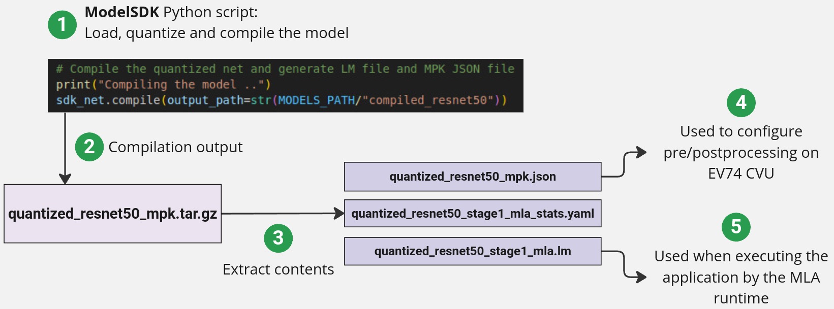
To better understand the contents of the *_mpk.json file, click the button below. While editing this file is typically unnecessary, reviewing its content can provide insight into the internals of the inferencing pipeline.

View